logo

Project AGI

Building an Artificial General Intelligence

This site has been deprecated. New content can be found at https://agi.io

Wednesday 24 December 2014

Sparse Distributed Representations (SDRs)

TL;DR:

  • An SDR is a Sparse Distributed Representation, described below
  • SDRs are biologically plausible data structures
  • SDRs have powerful properties
  • SDRs have received a lot of attention recently
  • There are a few really great new resources on the topic:

Background

An SDR is a binary vector, where only a small portion of the bits are ‘on’. There is growing evidence that SDRs are a feature of biological computation, for storing and conveying information. In a biological context, this represents a small number of active cells in a population of cells. SDR’s have been adopted by HTM (in CLA), and HTM's focus on this has set it apart from the bulk of mainstream machine learning research.

SDRs have very promising characteristics and are still relatively under utilised in the field of AI and machine learning. It’s an exciting area to be watching as AGI leaps forward.

The concept of SDRs are not new however. Kanerva first proposed a sparse distributed memory as a physiologically plausible model for human memory in his influential 1988 book Sparse Distributed Memory [Kanerva1988]. The properties of sparse distributed memory were nicely summarised by Denning in 1989 [Denning1989].

As early as 1997, Hinton and Ghahramani described a generative model, implementable with a neural network, that ‘discovered’ sparse distributed representations for image analysis [Hinton1997].

Then in 1998 SDRs were used in the context of robot control for navigation by both Rajesh et. al and Rao et. al [Rajesh1998, Rao1998] and then in 2004 for reinforcement learning by Ratitch [Ratitch2004].

Recently some great new resources have become available. There is a new video from Numenta of Subutai Ahmad presenting on the topic. A nice companion to that is an older introductory video of Jeff Hawkins presenting. The recent draft paper by Ferrier on a universal cortical algorithm (discussed in an earlier blog post) gives an excellent summary of their characteristics.

What’s all the fuss about? - SDR Characteristics

Given that so much great (and recent) material exists describing SDRs, I won’t go into very much detail. This post would not be complete though, without at least a cursory look at the ‘highlights’ of SDRs.
  • Semantic
    • each bit corresponds to something meaningful
  • Efficient/Versatile
    • storage: there is a huge number of potential encodings for a given vector size, as capacity increases exponentially with number of potentially active bits
    • compositionality: because of sparsity SDRs are generally linearly separable and can therefore be combined to represent a set of several states
    • comparisons: it is very efficient to measure similarity between vectors (you just need to count overlap of ‘on’ bits) and if a state is part of a set (due to compositionality)
  • Robust
    • subsampled or noisy vectors are still semantically similar and can be compared effectively

Conclusion

We believe that these elements make SDRs an excellent choice as the main data structure of any AGI implementation - they are used in our current approach. The highlights and links given above should be a good start to anyone that wants to learn more.

Monday 22 December 2014

Agency and Hierarchical Action Selection

This post asks some questions about the agency of hierarchical action selection. We assume various pieces of HTM / MPF canon, such as a cortical hierarchy.

Agency

The concept of agency has various meanings in psychology, neuroscience, artificial intelligence and philosophy. The common element is having control over a system, with varying qualifiers regarding the entities who may be aware of execution or availability of control. Although "agency" has several definitions, let's use this one I made up:

An agent has agency over a state S, if its actions affect the probability that S occurs.

Hierarchical Selection thought experiment

Now let's consider a hierarchical representation of action-states (actions and states encoded together). Candidate actions can therefore be synonymous with predictions of future states. Let's assume that actions-states can be selected as objectives anywhere in the hierarchy. More complex actions are represented as combinations or sequences of simpler action-states defined in lower levels of the hierarchy.

Let's say an "abstract" action-state at a high level in the hierarchy is selected. How is the action-state executed? In other words, how is the abstract state made to occur?

To exploit the structure of the hierarchy, let's assume each vertex of the hierarchy re-interprets selected actions. This translates a compound action into its constituent parts.

How much control does higher-level selection exert over lower-level execution? For simplicity let's assume there are two alternatives:

1. High level selection biases or influences lower level (weak control)
2. Lower levels try to interpret high level selections as faithfully as possible (strong control)

We exclude the possibility that higher levels directly control or subsume all lower levels due to the difficulty and complexity of performing such a task without the benefit of hierarchical problem decomposition.

If high levels do not exert strong control over lower levels, the probability of faithfully executing an abstract plan should be small due to compound uncertainty at each level. For example, let's say the probability of each hierarchy level correctly interpreting a selected action is x. The height of the hierarchy h determines the number of interpretations between selection of the abstract action and execution of relevant concrete actions. The probability of an abstract action a being correctly executed is:

P(a) = xh

So for example, if h=10 and x=0.9, P(a) = 0.34.

We can see that in a hierarchy with a very large number of levels, the probability of executing any top-level strategy will be very small unless each level interprets higher-level objectives faithfully. However, "weak control" may suffice in a very shallow hierarchy.

Are abstract actions easy to execute?

Introspectively I observe that highly abstract plans are frequently and faithfully executed without difficulty (e.g. it is easy to drive a car to the shops for groceries, something I consider a fairly abstract plan). Given the apparent ease with which I select and execute tasks with rewards delayed by hours, days or months, it seems I have good agency over abstract tasks.

According to the thought experiment above, my cortical hierarchy must either be very shallow or higher levels must exert "strong control" over lower levels.

Let's assume the hierarchy is not shallow (it might be, but then that's a useful conclusion in its own right).

Local Optimisation

Local processes may have greater biological validity because they imply less difficulty/specificity routing relevant signals to the right places. Hopefully the amount of wiring is reduced also.

What would a local implementation of a strong control architecture look like? Each vertex of the hierarchy would receive some objective action-state[s] as input. (When no input is received, no output is produced). Each vertex would produce some objective action-states as output, in terms of action-states in the level below. The hierarchical encoding of the world would be undone incrementally by each level. 

At the lowest level the output action-states would be actual motor control signals.

A cascade of incremental re-interpretation would flow from the level of original selection down to levels that process raw data (either as input or output). In each case, local interpretation should only be concerned with maximizing the conditional probability of the selected action-state given the current action-state and instructions passed to the level immediately below. 

Clearly, the agency of each hierarchy vertex over its output action-states is crucial. The agency of hierarchy levels greater than 0 is dependent on faithful interpretation by lower levels. Other considerations (such as reward associated with output action-states) must be ignored, else the agency of higher hierarchy levels is lost. 

Cortex Layer 6

Connections form between layer 6 of cortex in "higher" regions and layer 6 in "lower" regions, with information travelling from higher (more abstract) regions towards more concrete regions (i.e. a feedback direction). Layer 6 neurons also receive input from other cortex layers in the same region. However, note that the referenced work disputes the validity of assigning directionality, such as "feed-back", to cortical layers.

Pressing on regardless, given some assumptions about cortical hierarchy, we can speculatively wonder whether the layer 6 neurons embody a local optimization process that incrementally translates selected actions into simpler parts, using information from other cortex layers for context. The purpose of cortex layer 6 remains mysterious.

However, since cortex layer 5 seems to be the direct driver of motor actions, it may be that layer 6 somehow controls cortex layer 5 in the same or lower regions, perhaps via some negotiation with the Thalamus.

Adapted from Numenta CLA Whitepaper by Gideon Kowadlo
Another difficulty for this theory is that cortex layer 5 seems to be more complex than simply the output from layer 6. Activity in layer 5 seems to be the result of interaction between cortex and Thalamus. Potentially this interaction could be usefully overriding layer 6 instructions to produce novel action combinations.

There is some evidence that dopaminergic neurones in the Striatum are involved in agency learning, but this doesn't necessarily refute this post, because this process may modulate cortical activity via the Thalamus. Cortex layer 6 may still require some form of optimization to ensure that higher hierarchy levels have agency over future action-states.

To conclude: This is all speculation - comments welcome!

Tuesday 25 November 2014

Toward a Universal Cortical Algorithm: Examining Hierarchical Temporal Memory in Light of Frontal Cortical Function

This post is about a fantastic new paper by Michael R. Ferrier, titled:


Toward a Universal Cortical Algorithm: Examining Hierarchical Temporal Memory in Light of Frontal Cortical Function


The paper was posted to the NUPIC mailing list and can be found via:


The paper itself is currently hosted at:


It isn't clear if this is going to be formally published in a journal at some point. If this happens we'll update the link.


So, what do we like about this paper?

Purpose & Structure of the paper

The paper is mostly a literature review and is very well referenced. This is a great introductory work to the topic.


The paper aims to look at the evidence for the existence of a universal cortical algorithm - i.e. one that can explain the anatomical features and function of the entire cortex. It is unknown whether such an algorithm exists, but there is some evidence it might. Or, more likely, variants of the same algorithm are used throughout the cortex.


The paper is divided into 3 parts. First, it reviews some relevant & popular algorithms that generate hierarchical models. These include Deep Learning, various forms of Bayesian inference, Predictive Coding, Temporal Slowness and Multi-Stage Hubel Wiesel Architectures (MHWA). I'd never heard of MHWA before, though some of the examples (such as convolutional networks and HMAX) are familiar.  The different versions of HTM are also described.


It is particularly useful that the author puts the components of HTM in a well-referenced context. We can see that the HTM/CLA Spatial Pooler is a form of Competitive Learning and that the proposed new HTM/CLA Temporal Pooler is an example of the Temporal Slowness principle. The Sequence Memory component is trained by a variant of Hebbian learning.


These ties to existing literature are useful because they allow us to understand the properties and alternatives to these algorithms: Earlier research has thoroughly explored their capabilities and limitations.


Although not an algorithm per se, Sparse Distributed Representations are explained particularly well. The author contrasts 3 types of representation: Localist (single feature or label represents state), Sparse and Dense. He argues that Sparse representations are preferable to Localist because the former can be gradually learnt and are more robust to small variations.

Frontal Cortex

The second part of the paper reviews the biology of frontal cortex regions. These regions are not normally described in computational theories. Ferrier suggests this omission is because these regions are less well understood, so they offer less insight and support for theory.


However these cortical areas are of particular interest because they are responsible for representation of tasks, goals, strategy and reward; the origin of goal-directed behaviour and motor control.


Of particular interest to us is discussion of biological evidence for the hierarchical generation of motor behaviour and output to motors directly from cortex.

Thalamus and Basal Ganglia

The paper discusses the role of the Thalamus in gating messages between cortical regions, and discusses evidence that the purpose of the Striatum and Basal Ganglia could include deciding which messages are filtered in the Thalamus.  Filtering is suggested to perform the roles of attention and control (this all perfectly matches our understanding of the same).


There is a brief discussion of Reinforcement Learning (specifically, Temporal-Difference learning) as a computational analogue of Thalamic filter weighting. This has been exhaustively covered in the literature so wasn't a surprise.

Towards a Comprehensive Model of Cortical Function

The final part of the paper links the computational theories to the referenced biology. There are some interesting insights (such as that messages in the feedback pathway from layer 5 to layer 1 in hierarchically lower regions must be "expanding" time; personally I think these messages are being re-interpreted in expanded time form on receipt).


Our general expectation is that feedback messages representing predicted state are being selectively biased or filtered towards "predicting" that the agent achieves rewards; in this case the biased or filtered predictions are synonymous with goal-seeking strategies.


Overall the paper does a great job of linking the "ghetto" of HTM-like computational theories with the relevant techniques in machine learning and neurobiology.

Monday 24 November 2014

Recent HTM projects

It's exciting to see growing interest and participation in the AGI community.
This is another brief post to share two examples. In this case, they both build on one approach to AGI, and that is HTM.

FXAI - Explorations Into Computational Intelligence
A blog that is pretty well described by the title. The author, Felix Andrews, has been focussing on HTM, implementing a version of CLA in Clojure that runs in the browser and follows Visualisation Driven Development. The latest post describes a new algorithm for selection of winning columns based on local rather than global inhibition. Global inhibition is one of the compromises that the NUPIC implementation makes in favour of computational performance.

My Attempt at Outperforming DeepMind's Atari Results
DeepMind's successes caused a big splash in the AI research community and tech industry in general. This blog by Eric Laukien documents progress of a project that, as the title suggests, has the goal of achieving better performance than DeepMind. His approach is to incorporate Reinforcement Learning with HTM to create an agent that can learn how to act in the world. This is the only other example we've seen of an MPF implementation that can take actions.

Sunday 9 November 2014

Cortical Learning Algorithms with Predictive Coding for a Systems-Level Cognitive Architecture

This is a quick post to link a poster paper by Ryan McCall, who has experimented with a Predictive-Coding / Cortical Learning Algorithm (PC-CLA) hybrid approach. We found the paper via Ryan writing to the NUPIC theory mailing list.

What's great about the paper is it links to some of the PC papers we mentioned in a previous post and covers all the relevant literature, with clear and detailed descriptions of key features of each method.

So we have Lee & Mumford, Rao and Ballard, Friston (Generalized Filtering)... It's also nice to see Baar's Global Workspace Theory and LIDA (a model of consciousness or, at least, attention).

Ryan has added a PC-CLA module to LIDA and tested robustness to varying levels of input noise. So, early days with the experiments but great start.

http://www.cogsys.org/papers/2013poster7.pdf 

Friday 17 October 2014

A Unifying View of Deep Networks and Hierarchical Temporal Memory


Browsing the NUPIC Theory mailing list, I came across a post by Fergal Byrne on the differences and similarities between Deep Learning and MPF/HTM. It's a great background into some of the pros and cons of each.

Given the popularity and demonstrated success of Deep Learning methods it's good to understand how they work and how they relate to MPF/HTM theory. For example, both involve construction of hierarchical data representations created via a series of unsupervised classifiers. Fergal rightly admonishes proponents of both methods for their reluctance to research the alternatives!

The article can be found here:

http://inbits.com/2014/09/a-unifying-view-of-deep-networks-and-hierarchical-temporal-memory/

Thursday 9 October 2014

On Predictive Coding and Temporal Pooling

Introduction

Predictive Coding (PC) is a popular theory of cortical function within the neuroscience community. There is considerable biological evidence to support the essential concepts (see e.g. "Canonical microcircuits for predictive coding" by Bastos et al).

PC describes a method of encoding messages passed between processing units. Specifically, PC states that messages encode prediction failures; when prediction is perfect, there is no message to be sent. The content of each message is the error produced by comparing predictions to observations.

A good introduction to the various theories and models under the PC umbrella has been written by Andy Clark ("Whatever next? Predictive brains, situated agents, and the future of cognitive science"). As Clark explains, the history of the PC concept goes back at least several decades to Ashby, quote: "The whole function of the brain is summed up in: error correction." Mumford pretty much nailed the concept back in 1992, before it was known as predictive coding (the cited paper gives a good discussion of how the neocortex might implement a PC-like scheme).

The majority of PC theories also model uncertainty explicitly, using Bayesian principles. This is a natural fit when providing explicit messaging of errors and attempting to generate predictions. Of course, it is also a robust framework for generative models.

It can be difficult to search for articles regarding PC because a similar concept exists in Signal Processing, although this seems to be coincidental, or at least the connection goes back beyond our reading. Unfortunately, many articles on the subject are written at a high level and do not include sufficient detail for implementation. However, we found work by Friston et al (example) and Rao et al (example, example) to be well described, although the former is difficult to grasp if one is not familiar with dynamical systems theory.

Rao's papers include application of PC to visual processing and Friston's work includes both the classification of birdsong and extends the concept to the control of motor actions. Friston et al wrote a paper titled "Perceptions as hypotheses; saccades as experiments" in which they suggest that actions are carefully chosen to optimally reduce uncertainty in internal predictive models. The PC concept throws up interesting new perspectives on many topics!

Comparison to MPF/CLA

There are significant parallels between MPF/CLA and PC. Both postulate a hierarchy of processing units with FeedForward (FF) and reciprocal FeedBack (FB) connections. MPF/CLA explicitly aims to produce increasingly stable FF signals in higher levels of the hierarchy. MPF/CLA tries to do this by identifying patterns via spatial and temporal pooling, and replacing these patterns with a constant signal.

Many PC theories create "hierarchical generative models" (e.g. Rao and Ballard). Hierarchical is enforced by restrictions on the topology of the model. The generative part refers to the fact that variables (in the Bayesian sense), in each vertex of the model, are defined by identification of patterns in input data. This agrees with MPF/CLA.

Both MPF/CLA and PC posit that processing units use FB data from higher layers to improve local prediction. In conjunction with local learning, this serves to reduce errors and therefore, in PC also stabilizes FF output.

In MPF/CLA it is assumed that cells' input dendrites determine the set of inputs the cell represents. This performs a form of Spatial Pooling - the cell comes to represent a set of input cells firing simultaneously, and hence the cell becomes a label or symbol representing that set. In PC it is similarly assumed that the generative model will produce objects (cells, variables) that represent combinations of inputs.

However, MPF/CLA and PC differ in their approach to Temporal Pooling, i.e. changes in input over time.

Implicit Temporal Pooling

Predictive coding does not expressly aim to produce stability in higher layers, but increasing stability over time is an expected side-effect of the technique. Assuming successful learning within a processing unit, its FF output will be stable (no signal) for the duration of any periods of successful prediction.

Temporal Pooling in MPF/CLA attempts to replace FF input with a (more stable) pattern that is constantly output for the duration of some sequence of events. In contrast, PC explicitly outputs prediction errors whenever they occur. If errors do not occur, PC does not produce any output, and therefore the output is stable. A similar outcome has occurred, but via different processes.

Since the content of PC messages differs to MPF/CLA messages, it also changes the meaning of the variables defined in each vertex of the hierarchy. In MPF/CLA the variables will represent chains of sequences of sequences ... in PC, variables will represent a succession of forks in sequences, where prediction failed.

So it turns out that Predictive Coding is an elegant way to implement Temporal Pooling.

Benefits of Predictive Coding

Where PC gets really interesting is that the amplitude or magnitude of the FF signal corresponds to the severity of the error.  A totally unexpected event will cause a signal of large amplitude, whereas an event that was considered a possibility will produce a less significant output.

This occurs because most PC frameworks model uncertainty explicitly, and these probability distributions can account for the possibility of multiple future events. Anticipated events will have some mass in the prior distribution; unanticipated events have very little prior probability. If the FF output is calculated as the difference between prior and posterior distributions, we naturally get an amplitude that is correlated with the surprise of the event.

This is a very useful property. We can distribute representational resources across the hierarchy, giving the resources preferentially to the regions where larger errors are occurring more frequently. These events are being badly represented and need improvement.

In biological terms this response would be embodied as a proliferation of cells in columns receiving or producing large or frequent FF signals.

Next post

In the next post we will describe a hybrid Predictive-Coding / Memory Prediction Framework which has some nice properties, and is appealingly simple to implement. We will include some empirical results that show how well the two go together.


Saturday 2 August 2014

Some experimental results with NUPIC

A quick post here to give readers an idea of HTM/CLA performance on visual object recognition tasks.

Although a little out of date now, Craig's blog gives a good idea of what NUPIC can and can't do, and how data issues (e.g. training set, variations in object appearance) affect the results. This is a handy review for someone considering working with NUPIC:

http://www.craigquiter.com/post/16984424066/htm-notes


Wednesday 2 July 2014

Connectome browser - hierarchy viewer?

Hierarchy Viewer?


Ongoing research to map out the patterns of connectivity in the human brain continues to produce stunning visuals. Are we looking at the hierarchy as proposed in the Memory-Prediction framework?

In any case, it's fun to explore, which you can do here:

http://www.humanconnectomeproject.org/data/relationship-viewer/


Wednesday 25 June 2014

TP 3/3: Proposed Temporal Pooler

by David Rawlinson and Gideon Kowadlo

A Temporal Pooler Proposal
We will describe a Temporal Pooler design below. We have tested this design and it gives satisfactory output given the criteria and expectations described below and in the previous articles in this series (post #1, post #2). It is also relatively simple. You could imagine this design being implemented in biology, but we have no biological evidence that this is the design used in the cortex. Nevertheless, it is useful to have a template for an "ideal" design (from a certain perspective), against which to compare known biology.

[EDIT: We have now rejected this design and prefer temporal pooling via on Predictive Coding]

This article will first list our design criteria, then give pseudocode for the TP implementation. Finally we will work through some examples to show the output of our temporal pooler.

Assumptions
1. This is a design based on engineering requirements, not based on biology

2. For simplicity of explanation, we will assume a "Region" is a piece of cortex comprising several layers of cells with distinct functions. There is mutual inhibition and high internal connectivity within the region. The region has a finite 2-d extent within all layers.

3. For a given set of active feed-forward (FF) input cells (let's call this an input "pattern"), each sub-region will have a single "winning" spatial-pooler (SP) cell that most closely matches the input pattern. This differs from the CLA/HTM definition of a region, where there may be multiple "winners". However, for this example let's keep things simple.

4. The finite set of cells local to the region mean that all configurations of world and agent are represented by states in a small, loopy graph embodied by the region's SP cells. "Loopy" means that there is at least one cycle and that there are no terminal states in this digraph. We understand that the local representation of agent + world state will be missing a lot of detail, that that's OK.

5. The temporal pooler will only update on a change to the FF input pattern.

6. Temporal Pooling should guarantee to increase output stability for any given sequence of SP cell activation. This means that sequences of length at least 3 must be replaced with constant output from the Temporal Pooler.

7. Uncertainty should not be hidden by the Temporal Pooler. Where forks occur in the graph, TP output should change, unless the fork is predictable. If an unpredicted event occurs, TP output should change to allow the transition to be modelled at a higher hierarchy level.

8. We assume that state-splitting creates redundant SP-cells that respond to the same FF input, but with different prior (previous) cell activations. e.g. SP cell #1 responds to uniquely to "green" after "blue", and SP cell #2 responds to "green" after "red". See the earlier post for more on this. A combination of state-splitting and simultaneous multiple TP-cell activation is necessary to guarantee pooling. It also allows variable-order modelling of FF input in different sequential contexts.

Outline
We require 2 sets of cells for our design. First, a layer of SP cells. A single SP cell fires for a given FF input, and represents the observation of that input when active.

Second, a layer of TP cells. We require 1 TP cell per SP cell. While SP cells fire individually, and only one at any given time, a set of TP cells will be simultaneously active. The set of active TP cells collectively represent a sequence of FF input, and the set must collectively fire only on observation of a specific and unique sequence of active SP cells. In a hierarchy, the next layer's SP cells will replace the active TP cells with individual cells that represent these combinations.

At all times at least 1 TP cell will be active.

The design has 2 key elements:
- Propagation of TP cell activity based on first-order modelling of historical transitions between SP cells.
- Assumes state splitting has created redundant SP cells representing the same FF input patterns, thereby allowing variable-order modelling using only first-order relations between SP cells.
- Inhibition of TP cell activity after a prediction failure.

Pseudocode
Variables:
nCells: The number of SP and TP cells
spCells: An array of SP cell activation values, length nCells
inCells: An array of TP cell inhibition values, length nCells
tpCells: An array of TP cell activation values, length nCells
spBest: The winning SP cell that matches the current FF input
spPrev: The previous winning SP cell.
spPred: The SP cell predicted to be the next best cell.
w( i, j ): Probability of transition from SP cell i to SP cell j in local graph

Note that weights w(i,j) represent conditional probabilities w(i,j) = P( S'=j | S=i ) where S is the currently active SP cell and S' is the next active SP cell. The weights can be approximated using historical observations of transition frequencies between active SP cells. Learning of sequence memory transitions is not covered in the pseudocode below. Similarly, the process for learning and defining the set of SP cells is not described.

// clear tp cell activity after bad prediction
if( spPred != spBest ) { // last prediction wrong
  inCells[ spPrev ] = 1;
  tpCells[ all ] = 0;
}

// clear tp cell activity when we reach inhibited cell
if( inCells( spBest ) ) {
  tpCells[ all ] = 0;
}

// clear inhibition of winning cell and activate it
inCells[ spBest ] = 0
tpCells[ spBest ] = 1

// now propagate this activity forwards
sp1 = spBest;

int i = 0;
while( i < nCells ) { // or stop when stable

  sp2Max = null;
  wMax = 0;

  // find the most likely transition starting at sp1
  for( sp2 = 0; sp2 < nCells; ++sp2 ) {
    if( sp1 == sp2 ) continue;
      
    if( w( sp1, sp2 ) > wMax ) {
      wMax = w( sp1, sp2 )
      sp2Max = sp2;
    }
  }

  // check inhibition, and consider replacing 
  // sp1 with sp2Max to continue propagation.
  if( sp2Max != null ) {
    if( inCell[ sp2Max ] > 0 ) {
      break; // don't propagate to this cell, it is inhibited
    }
    else { // not inhibited
      tpCells[ sp2Max ] = 1; // activate
      sp1 = sp2Max; // now project forward from here
    }
  }

  ++i;
}

So what does it do?
Let's work through a simple example that includes deterministic sequences and a non-deterministic fork. Obviously, the latter cannot always be predicted.

Figure 1: First order (left) and variable order via state-splitting (right) representations of a problem. The problem is characterized by observation of a colour in each state. There are 7 states (some colours occur in more than 1 state). The 7 states are organised into 2 sequences (R,G,B and G,B,R). After state 1 (black), a random sequence is chosen.

Figure 1 shows a test problem where each state has a corresponding colour observation. Four different colours are observed (red, green, blue and black). Arrows indicate transitions between states. The "true" graph of the problem is shown to the right. On the left is a first-order graph of observations. State-splitting is necessary to build a more useful model of the transitions between states, creating redundant copies of states with red, green and blue observations. Let's just assume that the SP cells have formed the "correct" representation of the world shown (figure 1, right) because that learning process is too complex to explain here. The fork at state 1 is random, with a slight bias making transition from 1 to 2 more likely than from 1 to 5. State 1 is shown twice for improved presentation.

Figure 2: Key for diagrams used in the rest of this post. We have 2 sets of cells: TP cells (left column styles) and SP cells (right column styles).

Figure 2, above, shows the annotations and styling we use to present the state of SP and TP cells in the following walkthrough of the proposed temporal pooling algorithm.

Figure 3: SP cell 1 is active. Each SP cell has an associated TP cell (none active yet).

Figure 3: Say that via state-splitting, we have constructed a set of 7 SP cells (centre graph, coloured and numbered circles). This means we also need to create 7 TP cells (we specified earlier that there would be 1 TP cell per SP cell). Each TP cell is associated with one SP cell. The magenta outline of SP cell 1 indicates that this cell has been selected as best matching the current FF input. None of the TP cells are active. The heavier arrow from SP cell 1 to 2 represents the higher probability of this outcome.

Figure 4: TP cells active via prediction.

Figure 4: According to the algorithm given above, we will first activate TP cell 1 due to activity of SP cell 1 (magenta). Then, we propagate forwards the activation through TP cells 2,3,4 because this is the most likely path (brown outline highlights). Activation propagates back to TP cell 1 and then has no further effect, since TP cell 1 is already active. TP cells 5,6,7 are not activated because this is not the most likely path from TP cell 1. As a result, of our 7 TP cells, 4 are active {1,2,3,4} of {1,2,3,4,5,6,7}.

Figure 5: Remember activation of TP cell 1. 

Figure 5: The external world moves from a state generating the black observation, to green. SP cell 2 is correspondingly made active. The temporal pooler cells are now updated, starting by activating TP cell 2 (although it is already active). TP cell 1 remains active for two reasons: First, activity is not cleared unless there is a prediction failure. Second, activity propagates from TP cell 2 through TP cells 3,4, and 1, back to 2. Again, TP cells 5,6,7 are not active. There has been no change in the set of active TP cells as they are following a predictable sequence. In fact, the set of active TP cells will not change while visiting any of the active states {1,2,3,4}.

Figure 6: Prediction failure. We predicted a transition from SP cell 1 to 2, but observed from 1 to 5. Inhibit activation of TP cells associated with SP cell 1.

Figure 6: If, randomly, a transition from SP cell 1 to SP cell 5 occurs, the pattern of TP cell activation will change. TP cell 1 will be inhibited (magenta X) due to the prediction failure. TP cell 5 will be activated and the activity will propagate through TP cells 6 and 7. Crucially, it cannot propagate further due to inhibition of TP cell 1. This prevents the set of active cells extending to TP cells 2,3,4.

Figure 7: TP cell 5 activity remembered. TP cell 6 directly activated by SP cell 6. TP cell 7 activated by prediction. TP cell 1 inhibited.

Figure 7: For the remainder of the sequence R-G-B, TP cells 5,6,7 remain active. While Green is observed, as shown above, TP cell 5 remains active not due to forward prediction but due to the fact that TP cell activity is retained until there is a prediction failure.

Discussion
In this example, TP output is one of two subsets of cells, either {1,2,3,4} or {5,6,7}. In the next hierarchy layer, the active subsets would be associated with specific SP cells that would represent these sequences of observations in their entirety.

This is a relatively simple scheme that only requires inhibition and prediction. A prediction failure is always followed by a change in TP output, due to the inhibition mechanism, even if the most likely path leads back to the original set of active cells prior to the failed prediction. Recall that the local graph being modelled in a region of cortex will always feature cycles and have no terminal states. Without inhibition, we would end up with scenarios where all TP cells were constantly active regardless of which fork was taken (if a lower-probability outcome occurs). This would obscure the unpredictable transitions and make them unavailable for modelling higher in the hierarchy.

At least 1 TP cell is always active (the cell that is associated with the currently active SP cell).

The output of the temporal pooler is maximally stable when sequences of observations are predictable. This is ideal if we assume the predicted outcome is the most common outcome. The propagation mechanism as proposed makes best use of predictable transitions - sequences of arbitrary length can be replaced with a constant output, if the system is sufficiently predictable.

Note that this method can only guarantee to simplify the observed problem in combination with state-splitting. The latter is required to build more and longer deterministic sequences of SP cell activation, even if these sequences are not predictable. It is assumed that given increasingly higher-order interpretation, predictability will be achieved.

In a future post we will look in more detail about the process of state-splitting.

Saturday 31 May 2014

TP 2/3: Jeff's new Temporal Pooler

By David Rawlinson and Gideon Kowadlo

Jeff's new Temporal Pooler

This is article 2 in a 3 part series about Temporal Pooling (TP) in MPF/CLA-like algorithms. You can read part 1 here. For the rest of this article we will assume you've read part 1.

This article is about the new TP proposed by Jeff Hawkins. The original TP was described in the CLA white paper. We will also assume you've at least had a quick read of the linked articles. Despite our best efforts this article is only an interpretation of those methods, and it may not be entirely correct or as Numenta intended.

Separation of internal and external causes

The first topic in Hawkins' proposal covers the possible roles of specific cortical layers and the separation of internal and external causes.

Hawkins suggests that cortical layers 3,4,5 and 6 are all implementing variants of the same algorithm, with minor differences. He also suggests that each layer is performing all functions (Spatial Pooling, Sequence Memory and Temporal Pooling. In higher hierarchy levels, Spatial Pooling may be absent). In CLA, these 3 components are implemented as a matrix of sequence-memory cells. Rules concerning how and when the cells activate each other in different input contexts implement the pooling and prediction features.

Hawkins also states that one distinction between layers 3 and 4 may be that cells in layer 4 are using copies of motor actions (internal causes), to predict better. In consequence, cells in layer 3 are left trying to predict the actions that layer 4 could not predict, i.e. relying more on historically-observed sequential patterns of activation. Although both layers will learn sequential patterns of activation, layer 3 will rely more heavily on history. External causes will more often generate input that can’t be explained by motor actions, so we might expect layer 3 to more often respond to external events.

This article will not discuss these ideas any further. We note them for clarity and to distinguish our focus. Instead, we will talk about how the new CLA TP could be used to construct a hierarchical representation of changes in input patterns over time.

Temporal Slowness

Both old and new temporal poolers exploit a principle known as "Temporal Slowness", which means that output activity varies more slowly than input activity. You can read more about this general principle here.

Another, related feature of the HTM and CLA temporal poolers is that they emit a constant pattern of cell activity to generate stability. This is achieved by marking cells as "active" regardless of whether they are active via prediction or via feedfoward input. Although active-by-prediction and active-by-FF-input are distinguished within the region for learning purposes, this distinction is not visible to the next higher region in the hierarchy.

Old Temporal Pooler Cell Activity

For reference, this is an outline of the TP functionality in the "old" TP from the Numenta CLA white paper.

The diagrams in this article each have 3 parts. At the top is a graph showing a fragment (in graph terminology, a component) of the Sequence Memory encoded by the cells in the region. Arrows show the learnt transitions between cells. Below the graph is a series of observations (marked "FF input") and the corresponding pattern of cell activity when each Feed-Forward (FF) input is observed. Each column represents a single cell from the sequence memory and its activity over time. Each row in the lower part of the diagrams shows all cells' activity at one moment. Cells are filled white when they are active and black when not active:


Figure 1: Spatial pooler and temporal pooler cell activity in the original CLA white paper. This image compares two patterns of cell activity over time, shown left and right. The left subfigure shows cell activity in spatial pooler cells, where the active cell[s] are the ones whose input bits most closely match current FF input. The right subfigure shows the original CLA temporal pooling method, where cells become active when predicted far in advance of their FF input being observed, and remain active until after the associated FF input is observed. In this example, ⅔ of the active cells are identical after each FF input change. A ‘P’ denotes cells activated due to prediction. Each subfigure has 3 parts. The main part is a matrix showing sequence memory cell activity over time. Each row is one time-step, numbered 1 to 5. The FF input observed at each time step is shown in a column to the left. The top row shows a fragment of Sequence Memory formed by the cells, and the colours each cell responds to. In this simple example, the Sequence Memory graph is simply a sequence of states that are always observed in the same order.
Spatial Pooler cell activity is easiest to explain (figure 1, left). In figure 1, we see that the Sequence Memory has learnt that the colours Red, Yellow, Green, Blue and Black occur in order. One cell responds uniquely to each of these colours, creating the diagonal line of active cells over time. Each cell is only active for the duration of its FF input being observed.

The original temporal pooler premise was to drive cells to an active state via prediction (cells active via prediction are marked with a 'P') as early as possible. The cells would then remain active until either the prediction was no longer made (e.g. due to observation of an unexpected FF input pattern) or the cell becomes active via its FF input.

Time and Stability

You can see in the figure above that in a sequence of predictable inputs each cell is active over a period of 3 input changes (the only meaningful way to measure time in these examples). So let's assume each input change is one time step.

The cells are shown to be active for an arbitrary period of time - to keep the diagrams simple the minimum period is shown. In reality a fixed activation period is unlikely; it will depend on the activation or prior cells in the sparse distributed representation. However, it is still possible to make the point that at any time during a predictable sequence, a set of cells is active. Most of those cells are not changing between time steps and will be active after the next FF input change. This is the temporal pooler in action.

In the example above, each cell is predicted up to 2 steps before the corresponding input is observed. Therefore, in a predictable sequence 3 cells are simultaneously active, 2 of them due to prediction and one due to FF input.

Although the output of the temporal pooler is continuously changing, most of the active cells are not changed between inputs. In this case, 2/3 of the output is stable. With longer activation of TP cells, a larger fraction of the output becomes stable.

Noisy recognition and resource constraint assumptions

To simplify the problem observed by the next level in the hierarchy it is necessary to have cell activity changes in the lower level without corresponding cell activity changes in the higher level. Given that the TP output is continuously changing, how do we sometimes avoid cell activity changes in the higher level?

There are two parts to the answer. First, all cells' FF input are Sparse Distributed Representations (SDRs). These are large sets of input bits, of which only a few are active at any given time. The Spatial Pooler in CLA recognises FF inputs when only a fraction of the expected (synapsed) input bits are active. For example, a cell may become active from FF input when 80% of its FF input bits are active - any 80%. The set of active input bits can change while the cell is active. This means that cells' recognition is tolerant to noisy FF input.

Noisy recognition of TP output from lower hierarchy levels is one assumption necessary for increasing stability in higher levels. But this assumption is actually a useful feature, allowing classification to be tolerant to noise.

The other necessary assumption is a resource-constraint. If an infinite supply of cells were available, then after much slow learning every FF input pattern would have a dedicated cell (due to inhibition between cells). Cell activity changes would occur throughout the hierarchy after every input change, no matter how tiny. Obviously, resource constraints are physically necessary.

The finite size of a CLA region ensures that there aren't enough cells to represent each FF input pattern perfectly. Instead, some similar (probably successive) FF inputs will be represented by the same set of active cells (quantization error).

These are both very reasonable assumptions, but worth stating and understanding.

New Temporal Pooler Cell Activity

The new TP proposes that cells are only counted as active when confirmed by observation of the corresponding FF input, and that they stay active for a period of time after this:


Figure 2: Spatial pooler and temporal pooler cell activity as described by the new TP method. Each TP cell is active for a period of time after its corresponding FF input is observed. There may be no distinct SP or TP cells, but we show them separately to illustrate differences in activation behaviour.
This in itself doesn't change much, but because we are now building patterns forwards we can represent unpredicted events more accurately. Cells are no longer active until the corresponding FF input is observed or prediction is cancelled; instead they are never fully activated prior to the corresponding FF input. When a prediction error occurs, the results are immediate and lasting. Given noisy recognition of FF input, the old method would be more likely to have hidden prediction failures.

Temporal pooling “replaces” graph components (specifically sequences of vertices) with a single vertex that represents the component by being constantly active for the duration of those inputs. It is also worth noting that to simplify any graph, the minimum number of vertices in each replaced sequence is 3. In a temporal pooler, this means that the minimum number of FF input changes for which a predicted cell must remain active is 3. If temporal pooler output is constant for sequences of length 2, the next hierarchy level will encode transitions between cells instead of sequences of cells (i.e. no simplification or effective pooling has occurred).

Activity after a Successful Prediction

The new TP proposes that there are two cortical layers of cells. One layer of cells embodies the Spatial Pooler. The other layer forms the TP. In the TP layer, cells remain active for a long time after being successfully predicted in the SP layer, but for only a short time when not predicted in the SP layer.

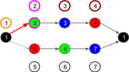
Prediction failures will occur regularly, whenever there are multiple future states and the available data does not allow the correct future to be determined. This looks like a fork in the Sequence Memory graph:

Figure 3: In this non-deterministic sequence, Red is followed by Yellow or Green. When the prior Red is observed, Yellow is predicted. Since it was predicted, the Yellow cell stays active for 3 steps in total. Since Blue always follows Yellow and Green, and Black follows Blue, the other cells are all active for the full 3 steps.
In the example above, the Yellow cell is successfully predicted leading to a long activation of the sequence memory cell that responds to Yellow after Red.

Activity after a Failed Prediction

The new TP proposes that in the event of a failed prediction, cells only remain active briefly. This is shown in the example below, where Yellow was predicted but Green was observed:

Figure 4: New TP cell activity after a failed prediction. Yellow was predicted but Green was observed.
The pattern of activity after a failed prediction is initially different to the pattern after a correct prediction, with only a short activation of the Green cell and no full activation of the predicted cell at all. This means that now, cells are only active when their corresponding FF input is actually observed.

The FF output of the TP after a prediction failure is quite different to the FF output during predictable sequences before and after. This helps to ensure that the unpredictable transition is modelled in higher hierarchy levels, passing the problem up the hierarchy rather than obscuring it. We anticipate that higher levels of the hierarchy will have the ability to understand and hence predict the problematic transition.

Analysis


Prediction with/without motor output distinguishes Cortex layers 3,4

Copying motor actions back to the cortex to help with prediction makes sense, especially in lower hierarchy levels. However, recent motor signals become increasingly irrelevant when trying to predict more abstract, longer term events. For example, getting sacked from your job is less likely due to the way you just now sipped your coffee, and more likely to do with some events that happened days or weeks ago. These older events will be hierarchically represented as more abstract causes.

At higher hierarchy levels, with greater abstraction, the "motor actions" that are necessary to explain & predict events are not simple muscle contractions, but complex sequences of decisions and behaviour with specific intents and expectations. The predictive data encoded in the Feed-Forward Indirect and Feed-Back (FB) pathways contains this data in a form that is appropriate and meaningful at each level of the hierarchy. If predictions and decisions are synonymous, then we can treat selected predictions as if they were actions.

For these reasons we are skeptical about the idea that the use of motor actions to aid prediction is enough to distinguish the functionality of different cortical layers. However, in support of the idea, layer 4 does disappear in higher hierarchy levels where motor actions would be less relevant.

Propagation of uncertainty to higher regions

The way that uncertainty (as prediction failure) is propagated up the hierarchy is vital to being able to reliably assemble a useful hierarchical representation of FF input. In fact, we believe that unpredictable events should be propagated until they reach a level of abstraction and invariance where they become predictable (see the Newtonian world assumption in the previous post). Therefore, we believe TP output should be highly orthogonal to prior and subsequent output in the event of a prediction failure. In the case of an SDR, highly orthogonal means that many bits should have dissimilar activity (a small intersection between the sets of active bits before and after).

Only a fraction of synapsed input bits are needed to activate a cell, and therefore CLA features “noise-tolerant” recognition of FF input. Only a few output bits would be dissimilar between the outcomes of prediction success and failure. This seems to raise the risk that unpredictable events could be “hidden” by noise-tolerance, and not passed up the hierarchy for higher levels to solve. From the perspective of a higher level, the set of active cells has not been significantly affected by their failure to predict.

Some loss of uncertainty in propagation may be acceptable in a sufficiently complex system. These are toy examples with only a few cells, whereas real CLA regions have hundreds or thousands of cells. However, we are working through some simple examples to try to better understand the behaviour and limits of the CLA.

Another detail that is not fully described in Hawkins’ current TP proposal is how long cells should be active when predicted. Maximum stability is achieved when cells are active for long periods, but we are limited by the conflicting objective to not hide uncertainty. Should we truncate activity when other prediction failures occur? In the next article we will propose explicitly making TP cells active unless uncertainty is too high, thereby implementing an auto-tuning of activation period.

Representations of random sequences

There is one comment in Hawkins' proposal that we disagree with. He says: "One of the key requirements of temporal pooling is that we only want to do it when a sequence is being correctly predicted. For example, we don't want to form a stable representation of a sequence of random transitions." In fact, it may be necessary to build a framework of some random sequences, in order to build sufficiently complex representations to explain any of the simpler events. Although the random sequences may not be the right ones, we need to have a mechanism of assembling more complex hierarchical representations even when there is no incremental explanatory power in doing so (this was discussed in the previous article). This would mean looking for structure in randomness, on the assumption that it would eventually be worthwhile due to explanatory models in higher levels of the hierarchy.

Summary

To wrap up:
- Feed-Back or Feed-Forward indirect pathway data may be a more appropriate source of data than motor actions in the FF direct pathway, for predicting events based on internal causes at higher levels of abstraction

- Reliable propagation of uncertainty (prediction failure) up the hierarchy is critical to move unexplained events to a level of abstraction where they can be understood

- We would like to extend activity period for maximum stability, balanced against the desire to avoid hiding prediction errors. How this is done is not detailed

- It may be necessary to perform temporal pooling even when there are no predictable patterns, in order to construct higher-order representations that may be able to predict the simpler events.

The next and final article in our 3 part series will present some specific alternative temporal pooler ideas.

Tuesday 27 May 2014

Thalamocortical architecture

by Gideon Kowadlo and David Rawlinson

Introduction

One of the keys to understanding the neocortex as a whole, and the emergence of intelligence, is to understand how the cortical hierarchical levels interconnect. This includes:
  • the physical connections,
  • the meaning of the signals being transmitted,
  • and possibly also the way the signal is encoded.
Physical connections: Physical connections refer to gross patterns of neuron routing throughout the brain. This is known as the connectome. Below is an image from the Human Connectome Project, that beautifully illustrates many connections including thalamocortical ones.
Figure 1. Courtesy of the Laboratory of Neuro Imaging and Martinos Center for Biomedical Imaging, Consortium of the Human Connectome Project - www.humanconnectomeproject.org

Meaning of signals: One classification that can be applied to thalamocortical neurons is drivers versus modulators. A driver can be thought of as a neuron that carries information, whereas a modulator modulates or alters the transmission of information in a driver. They have different functional and anatomical properties, as nicely described in (Sherman and Guillery 2011). If a neuron is a driver, what information does it encode, and if it is a modulator, is it inhibiting or excitatory and what effect does this have?

Signal Encoding: Signal encoding refers to the details of how the information is represented. This includes timing and amplitude information. The way the signal is encoded in the neurons may have a bearing on the properties of the system. Specific information has been added to the diagram where this looks relevant.

Our aim is to build AI with general intelligence characteristic of biological organisms such as primates. Therefore, we draw inspiration and insight from these working examples. Understanding the biology obviously gives us the best insight into how to do that. However, what level of abstraction do we need to capture the essential qualities?
  • at the lowest level: molecular structure, interactions and neurotransmitters,
  • above that, firing patterns and newly discovered molecular machinery (that excitingly shows this is more complex and interesting than previously thought - see paper and work by Seth Grant),
  • higher still, the brain as a set of modules that interact with each other,
  • or multi scale simulation of the whole brain (see the Human Brain Project).
For simplicity, we want to understand it at the highest level that is still capable of capturing the essential qualities, and drill down where necessary. Therefore, are factors such as the way that the signal is encoded important? Not in and of themselves, but they may have a bearing on emergent qualities, that are significant.

In order to understand the above, including drawing conclusions about the appropriate level of abstraction, we've elaborated on a figure first published in the CLA White Paper that was included in a previous post (in the section 'Regions'). In that article, we started to explore these topics in the context of Numenta's work. The figure shows the thalamo-cortical connections to specific cortical layers and is very useful for exploring the concepts described above. Here, we will expand on that figure, shown below. We will go over a first version, and we plan to make further posts in the future, as we develop it further. Each of the initial annotations are explained in the sub sections below.


Figure 2. Thalamocortical architecture including cortical layers and connections between hierarchy levels. This figure is an annotated version of a figure from the 'CLA White Paper'. Some information is added from the text of that document. Other sources used are Sherman and Guillery 2011Grossberg 2007, Sherman 2006 and Sherman 2007.


We invite the community to make use of and contribute to this annotated diagram. The diagram is publicly available in a universal vector graphics format called SVG. Being vector based, it is easily modifiable. SVG is a common format, which many graphics packages are capable of editing.

The file is available from a git repository hosted on github called cortico-thalamic-circuit. Anyone can download, clone, make a pull request or fork the repository.

Pull requests allow you to make modifications and then give them back to the shared repository so that they are available to everyone. This is the action to take if you share our purpose for the diagram - staying as high level as possible, filling in details where they contribute to a holistic view or emergent properties of the thalamocortical architecture. Forking allows you to create a new repository that diverges from the main one. Use this option if you’d like to use the diagram for a different purpose, such as documentation of all the neurotransmitters in the different pathways.

The first set of diagram additions are described below.

Diagram Additions

Cortico-Cortical Feedback

The illustrated feedback between levels from layer 6 in Level (n+1) to layer 1 in Level (n) is described briefly in the CLA white paper. We have included an additional illustration from Grossberg 2007 (see figure 3 below), that shows in more detail how internal neural circuitry completes the intra-cortical, inter-level, feedback loop from:

H[n+1]:C[6] → H[n]:d[1]C[5]
H[n]:d[1]C[5] → H[n]:C[6]
H[n]:C[6] → H[n]:C[4]

Note: The connections above are described in a notation we have adopted for succinctly describing cortical neural pathways. Refer to our post for more details.
Figure 3. Inter-level feedback loop, reproduced from Grossberg 2007. The circles and triangles are neuron bodies, with varying shape depicting different neuron types. Two hierarchy levels are shown (V1,V2 from the visual cortex). Each hierarchy level has 6 cortical layers (numbered 1 to 6 where relevant). You can see that feedback from V2 affects activation of neurons in V1 layer 4.
The feedforward/feedback architecture gives rise to at least three important qualities, the first of which has been explored in the MPF literature. They are described below, reproduced from Grossberg 2007:
  1. the developmental and learning processes whereby the cortex shapes its circuits to match environmental constraints in a stable way through time; 
  2. the binding process whereby cortex groups distributed data into coherent object representations that remain sensitive to analog properties of the environment; and 
  3. the attentional process whereby cortex selectively processes important events. 
We may elaborate with a summary of Grossberg 2007 in a future post.

Gating by the Thalamus

Our main references for this section are Sherman 2006 and Sherman 2007.

We've seen that the thalamus acts as a relay for information passing up the hierarchy between cortical levels, which we're referring to as the feedforward indirect pathway (FF Indirect). It has been postulated that via this gating, the thalamus plays an important role in attention.

What inputs and computations determine that gating? This is one of the questions we are attempting to learn more about, and so have explored inputs to the gating.

Cortical feedback

One of the significant inputs is FB from Layer 6 in the level above. That is to say that the gating from Level (n) to (n+1), is modulated by FB from Layer 6 in Level (n+1).

Thalamic feedback and TRN

There is a substructure of the Thalamus called the Thalamic Reticular Nucleus (TRN) that receives cortical and thalamic excitatory input, and sends inhibitory inputs to the relay cells of the thalamus.

These gating cells also receive inhibitory input from other Thalamic cells, labelled interneurons. Thalamic interneurons receive input from the very same relay cells, layer 6 of the cortex and the brainstem.

These circuits between TRN, BRF and thalamus are complex. They are simplified in the figure below, which appears in Sherman 2006 (Scholarpedia on the Thalamus), a version of which is found in Sherman 2007.

Figure 4. "Schematic diagram of circuitry for the lateral geniculate nucleus. The inputs to relay cells are shown along with the relevant neurotransmitters and postsynaptic receptors (ionotropic and metabotropic) Abbreviations: LGN, lateral geniculate nucleus; BRF, brainstem reticular formation; TRN, thalamic reticular nucleus." Caption and figure reproduced from Sherman 2006.

We are currently representing this complexity as a black box (as shown in the diagram) that receives input from the Thalamus, BRF and cortex, and inhibits the relay cells. The purpose and transfer function require analysis and exploration. It may be necessary to model the complexity explained above, or some simpler equivalent may provide the necessary functionality.

BRF

The BRF is the Brainstem Reticular Formation, which as the name suggests, is a part of the brainstem. It has a number of functions that could be very important for attention and general functioning of the cortex, and therefore, we have included it and it’s connections to the Thalamus. Some of these functions include:
  1. Somatic motor control
  2. Cardiovascular control
  3. Pain modulation
  4. Sleep and consciousness
  5. Habituation
The Wikipedia page for the BRF gives a very good summary.

Modulation Signal Characteristics

It is interesting to note that the firing mechanism for the BRF and Layer 6 modulation of the Thalamic relay is Burst Mode rather than the more common Tonic Mode. Tonic firing has a frequency that is proportional to the 'activation' of a neuron. The frequency can be interpreted as the "strength" of the signal. Some have interpreted it in the past as a probability or confidence value. For Burst Mode firing, after a 'silent' period, the initial firing pattern is a burst of activity. This "results in a very different message relayed to cortex, depending on the recent voltage history of the relay cell" (Sherman 2006). It is thought that this acts as a ‘wake up call’ to the cortex when there has been some external change. We plan to speculate and elaborate further on possible purposes of this in the future.

Timing Information

The CLA White Paper makes mention of timing information being fed back from the thalamus to layer 5 via layer 1. This has been added to the diagram for visibility. It is thought to be important for prediction of the next state at the appropriate time.

Other Factors

There are a number of other significant brain components that may substantially affect the operation of the neocortex. Based on the literature, the most significant of these is probably the Basal Ganglia, which forms circuits with the Thalamus and Cortex. Another interesting and possibly important component are Betz cells, which directly drive muscles from the cortex.

Conclusion

This post was a first attempt to create an enhanced diagram of cortical layers and thalamocortical connectivity in the context of MPF/HTM/CLA theory. We'll continue to elaborate on this in future posts.