TP 1/3: Temporal Pooler background

by David Rawlinson and Gideon Kowadlo

Article Series

This is the first of 3 articles about temporal pooler design for Numenta's Cortical Learning Algorithm (CLA) and related methods (e.g. HTM/MPF). It has limited relevance to Deep Belief Networks.

This first part will describe some of the considerations, objectives and constraints on temporal pooler design. We will also introduce some useful terminology. Part 2 will examine Jeff Hawkins' new temporal pooler design. Part 3 will examine an alternative temporal pooler design we are successfully using in our experiments.

We will use the abbreviation TP for Temporal Pooler to save repeating the phrase.

Purpose of the Temporal Pooler

What is the purpose of the Temporal Pooler? The TP is a core process in construction of a hierarchy of increasingly abstract symbols from input data. In a general-purpose algorithm designed to accept any arbitrary stream of data, building symbolic representations, or associating a dictionary of existing symbols with raw data, is an exceedingly difficult problem. The MPF/CLA/HTM family of algorithms seeks to build a dictionary of symbols by looking for patterns in observed data, specifically:

a) inputs that occur together at the same time
b) sequences of inputs that reliably occur one after another

The Spatial Pooler's job is to find the first type of pattern: Inputs that occur together. The TP's job is to find the second type of pattern - inputs that occur in predictable sequences over time. MPF calls these patterns "invariances". Repeated experience allows discovery of invariances: reliable association in time and space binds inputs together as symbols.

MPF/CLA/HTM claims that abstraction is equivalent to the accumulation of invariances. For example, a symbol representing "dog" would be invariant to the pose, position, and time of experiencing the dog. This is an exceptionally powerful insight, because it opens the door to an algorithm for automatic symbol definition.

What is a symbol? Symbols are the output of Classification. There must be consistent classification of the varying inputs that collectively represent a common concept, such as an entity or action. There must also be substitution of the input with a unique label for every possible classification outcome.

The symbol represents the plethora of experiences (i.e. input data) that cumulatively give the symbol its meaning. Embodiment of the symbol can be as simple as the firing of a single neuron. Symbols that represent a wider variety of input are more abstract; symbols that represent only a narrow set of input are more concrete.

Markov Chains

We will evaluate and compare TP functions using some example problems. We will be using Markov Chains to define the example problems. The Markov property is very simple; each state only depends on the state that preceded it. All information about the system is given by the identity of the current state. The current state alone is enough to determine the probability of transitioning to any other state.

Markov chains are normally drawn as graphs, with states being represented as vertices (aka nodes, typically presented as circles or ellipses). Changes in system state are represented by transitions between vertices in the graph. Edges in the graph represent potential changes, usually annotated with transition probabilities; there may be more than one possible future state from the current state. When represented as a Markov chain, the history of a system is always a sequence of visited states without forks or joins.

Here is an example Markov Chain representing a cycle of 4 states (A,B,C,D). Each state has a colour. The colour of the current state is observable. This graph shows that Red comes after Black. Green comes after Red. Blue follows Green, and Black follows Blue:

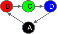
A simple Markov Chain shown as a graph. Vertices (circles) represent states. There are 4 states. Edges represent possible transitions between states. The color of each circle indicates what is observed in the corresponding state.

Now let's look at a more complex example. What happens when one state can be followed by more than one subsequent state? The answer is that the next state is determined randomly according to the probability of each transition.

A Markov chain with 7 states. State A can be followed by B or E with equal probability. Both states D and G are always followed by state A. This system represents 2 sequences of colours, separated by black. Each sequence is equally likely to occur, but once the sequence starts it is always completed in full.

In our examples, when there is a fork, all subsequent states are equally likely.  This means that in the example above, both states B and E are equally likely to follow state A.

First-Order Sequence Memory Representation

If we allow an MPF hierarchy to observe the system described by the Markov Chain above, the hierarchy will construct a model of it. Spatial pooling tries to identify instantaneous patterns (which will cause it to learn the set of observed colours). Temporal pooling attempts to find sequential patterns (frequently-observed sequences of colours). More simply put, an MPF hierarchy will try to learn to predict the sequences of colours.

How accurately the hierarchy can predict colours will depend on the internal model it produces. We know that the "real" system has 2 sequences of colours (RGB and GBR). We know that there is only uncertainty when the current state is Black.

However, lets assume the MPF hierarchy consists of a single region. Let's say the region has 4 cells, that learn to fire uniquely on observation of each of the 4 colours. The Sequence Memory in the region learns the order of cell firing - i.e. it predicts which cell will fire next, given the current cell. It only uses the current active cell to predict the next active cell.

The situation we have described above can be drawn as a Markov Chain like this:

A Markov chain constructed from first-order prediction given observations from the 7-state system shown in the previous figure. 

Note that the modelled system is less predictable than the "real world" system we were observing. We can still be sure that Blue always follows Green. But when we look at which colours follow Blue, we can only say that either Black or Red will follow blue. Similarly, we cannot predict whether Red will be followed by Green or Black, whereas in the "real" world this is predictable.

The reason for the lack of predictive ability is that we are only using the current colour of our model to predict the next colour. This is known as first-order prediction (i.e. Markov order=1). If we used a longer history of observations, we could predict correctly in every case except Black, where we could be right half the time. Using a "longer" history to predict is known as variable-order prediction (variable because we don't know, or limit, how much history is needed).

Uncertainty and the Newtonian experience

In today's physics, non-determinism (future not decided) or at least in-determinism (inability to predict) are widely and popularly accepted. But although these effects may dominate on very small and large scales, for much of human-scale experience the physical world is essentially a predictable, Newtonian system. Indeed, human perception encodes Newtonian laws so exactly that acceleration of objects induces an expectation of animate agency. 

In a Newtonian world, every action is "explained" or caused by some other physical event; it is simply necessary to have a sufficiently comprehensive understanding & measurement to be able to discover the causes of all observed events.

This intuition is important because it motivates the construction of an arbitrarily large hierarchy of symbols and their relations in time and space, with the expectation that somewhere in that hierarchy all events can be understood. It doesn't matter that some events cannot be explained; we just need to get enough practical value to motivate construction of the hierarchy. The Newtonian nature of our experiences at human scale means that most external events are comprehensible and predictable. 

Finding Higher-Order Patterns in Markov Chains

The use of longer sequences of colours to better explain (predict) the future shows that confusing, unpredictable systems may become predictable when more complex causes are understood. Longer histories (higher-order representations) can reveal more complex sequences that are predictable, even when the simpler parts of these patterns are not predictable by themselves.

The "Newtonian world" assumption gives us good reason to expect that a lot of physical causes are potentially predictable, given a suitably complex model and sufficient data. Even human causes are often predictable. It is believed that people develop internal models of third party behaviour (e.g. "theory of mind"), which may help with prediction. This evidence motivates us to try to discover and model these causes as part of an artificial general intelligence algorithm.

Therefore, one purpose of the MPF hierarchy is to construct higher-order representations of an observed world, in hope of being able to find predictable patterns that explain as many events as possible. Given this knowledge, an agent can use the hierarchy to make good, informed decisions.

Constructing Variable-Order Sequences using First-Order Predictions

There is one final concept to introduce before we can discuss some temporal pooler implementations. The final concept is ways of representing variable-order sequences of cell activation in a Sequence Memory. This is not trivial because the sequences can be of unlimited length and complexity, (depending on the data). However, for practical reasons, the resources used must be limited in some way. So, how can arbitrarily complex structures be represented using a structure of limited complexity?

Let's define a sequence memory as a set of cells, where each cell represents a particular state. Let's specify a fixed quantity of cells, and to encode all first-order transitions between these cells. All such pairwise transitions can be encoded in a matrix of dimension cells x cells. This means that cells only trigger each other individually; only pairs of cells can participate in each sequence fragment.

So, how can longer sequences be represented in the matrix? How can we differentiate between occurrences of the same observation in the context of different sequences?

The "state splitting" method of creating a variable-order memory using only first-order relationships between cells. This is part of a figure from Hawkins, George and Niemasik's "Sequence memory for prediction, inference and behaviour" paper. In this example there are 5 states A,B,C,D,E. We observe the sequences A,C,D and B,C,E. In subfigure (c), we see that for each state A,...,E there are a bunch of cells that respond to it. However, each cell only responds to specific instances of these states. Specifically, there are two cells (C1 and C2) that respond to state C. C1 responds to state C only after state A. C2 responds to an observation of state C only after state B. If we have only a single cell that responds to C, we lose the ability to predict D and E (see subfigure (d)). With two cells uniquely responding to specific instances of C (see subfigure (e)), we gain the ability to predict states D and E.  Prediction is improved by splitting state C, giving us a variable-order memory.

An elegant answer is to have multiple cells that represent the same observation, but which only fire in unique sequences. This concept is nicely explained in Hawkins, George and Niemasik's "Sequence memory for prediction, inference and behaviour" paper. They call it "state-splitting", i.e. splitting cells that represent an observed state and having multiple cells each responding to specific instances of the state in different sequences.

In the current CLA implementation, the same feature is achieved by having "columns" of cells that all respond to the same input in different sequence contexts (i.e. given a different set of prior cells). CLA says they share the same "proximal dendrite", which defines the set of input bits that activate the cell. In our paper, we showed how a radial inhibition function could induce sequence-based specialization of Self-Organising Map (SOM) cells into a variable-order sequence memory:

Creation of a variable order sequence memory in a Self-Organising Map (SOM) using inhibition. The circles represent cells that respond to the same input, in this case the letters A,B,C or D. We can use first-order sequence relationships to cause specialization of cells to specific instances of each letter. Blue lines represent strong first-order sequence relationships. The edge i-->k promotes k responding to "B" and inhibits x. Eventually k only responds to AB and x only responds to CB. 

In all cases, the common element is having multiple cells that respond to the same input, but only after specific sequences of prior inputs.

So, returning to our example problem above with 2 sequences of colours, RGB and GBR, what is the ideal sequence-memory representation using a finite set of cells, multiple cells for each input depending on sequence context, and only first-order relationships between cells? One good solution is shown below:

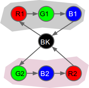
Example modelling of our test problem using a variable order sequence memory. We have 7 cells in total. Each cell responds to a single colour. Only one cell responds to black (BK). Having two cells responding to each colour R,G and B allows  accurate prediction of all transitions, except where there is genuine uncertainty (i.e. edges originating at black).  The temporal pooler component should then be able to identify the two sequences (grey and pink shading) by learning these predictable sequences of cell activations. The temporal pooler will replace each sequence with a single "label", which might be a cell that fires continuously for the duration of each sequence. Cells watching the temporal pooler output will notice fewer state changes, i.e. a more stable output.

Let's assume this graph of cells representing specific occurrences of each input colour (i.e. a Sequence Memory) provides the input to the Temporal Pooler. What is the ideal Temporal Pooler output?

Well, we know that there are in fact 2 sequences, and a "decision" state that switches between them. The ideal sequence-memory and temporal pooler implementation would track all predictable state changes, and replace these sequences with labels that persist for the duration of each sequence. In this way, the problem is simplified; other cells watching the temporal pooler output would observe fewer state changes - only switching between Black, Sequence #1 and Sequence #2.

Markov Chain that is experienced by an observer of the output from the ideal sequence-memory and temporal pooler modelling shown in the figure above. The problem has been reduced from 7 states to 3. State transitions are only observed when transitioning to or from the Black state (BK). Otherwise, a constant state is observed.

How can the ideal result be achieved? The next article will discuss how CLA simplifies sequences using the concepts described in this article, and the final article will discuss some alternative methods that we propose.

Architecture of the Memory Prediction Framework / Cortical Learning Algorithm / Hierarchical Temporal Memory

by David Rawlinson and Gideon Kowadlo

Introduction

The Memory Prediction Framework (MPF) is a general description of a class of algorithms. Numenta's Cortical Learning Algorithm (CLA) is a specific instance of the framework. Numenta's Hierarchical Temporal Memory (HTM) was an earlier instance of the framework. HTM and CLA adopt different internal representations so it is not as simple as CLA supersedes HTM.

This post will describe structure of the framework that is common to MPF, CLA and HTM, specifically some features that cause confusion to many readers.

For a good introduction to MPF/CLA/HTM see the Numenta CLA white paper.

The Hierarchy

The framework is composed as a hierarchy of identical processing units. The units are known as "regions" in CLA. The hierarchy is a tree-like structure of regions:

MPF/CLA/HTM hierarchy of Regions. The large arrows show the direction of increasing abstraction. Smaller arrows show the flow of data between nearby regions in a single level of the hierarchy, and between levels of the hierarchy. Figure originally from Numenta.

Regions communicate with other, nearby regions in the same level of the hierarchy. Regions also communicate with a few regions in a higher level of the hierarchy, and a few regions in a lower level of the hierarchy. Notionally, abstraction increases as you move towards higher levels in the hierarchy. Note that Hawkins and Blakeslee define abstraction as "the accumulation of invariances".

Regions

Biologically, each Region is a tiny patch of cortex. The hierarchy is constructed from lots of patches of cortex. Each piece of cortex has approximately 6 layers (there are small variations throughout the cortex, and the exact division between cortical layers in biology is a bit vague. Nature hates straight lines). Note that in addition to having only 6 layers, each cortical region is finite in extent within the cortex - i.e. it is only a tiny area on the surface of the cortex.

Cortical layers and connections between hierarchy levels. Each cortical region has about 6 structurally (i.e. also functionally) distinct layers. The hierarchy is composed of a tree of cortical regions, with connections between regions in different levels of the hierarchy. 3 key pathways are illustrated here. Each pathway is a carrier of distinct information content. The Feed-Forward pathways carry information UP the hierarchy levels towards increasing abstraction/invariance. The Feed-Back pathway carries information DOWN through hierarchy levels towards regions that represent more concrete, raw, unclassified inputs. Some pathways connect cortical regions directly, others indirectly (via other brain structures). Note that this image is a modified copy of one from Numenta, with additional labels and colours standardised to match the rest of this document.

Levels and Layers

Newcomers to MPF/CLA/HTM theory sometimes confuse "cortical layers" and connections between regions placed in different "levels" of the hierarchy. We recommend everyone uses layers to talk about cortical layers and levels to talk about hierarchy levels, although the levels and layers are somewhat synonymous in English. I believe this confusion arises because readers expect to learn one new concept at a time, but in fact levels and layers are two separate things.

Pathways

There are several distinct routes that information takes through the hierarchy. Each route is called a "pathway". What is a pathway? In short, a pathway is a set of assumptions that allows us to make some broad statements about what components are connected, and how. We assume that the content of data in each pathway is qualitatively different. We also assume there is limited mixing of data between pathways, except where some function is performed to specifically combine the data.

Directions

There are two directions that have meaning within the MPF/CLA/HTM literature. These are feed-forward and feed-back.  Feed-Forward (FF) means data travelling UP between hierarchy levels, towards increasing abstraction. Feed-Back (FB) means data travelling DOWN between hierarchy levels, with reducing abstraction and taking on more concrete forms closer to raw inputs.

3 Pathways

The 3 pathways typically discussed in the MPF/CLA/HTM literature are:

- FF direct (BLUE)

- FF indirect (GREEN)

- FB direct (RED)

Direct means that data travels from one cortical region to another, without a stop along the way at an intermediate brain structure. Indirect means that the data is passed through another brain structure en-route, and possibly modified or gated (filtered).

This does not mean that other pathways do not exist. There is likely a FB-indirect pathway from Cortex to Cortex via the Basal Ganglia, and direct connections between nearby Regions at the same level in the hierarchy. However, current canonical MPF/CLA theory does not assign roles to these pathways.  

We will always use the same colours for these pathways.

The conceptual and biological arrangement of the MPF/CLA/HTM hierarchy. Left, the conceptual structure. Right, the physical arrangement of the hierarchy. Cortical processing occurs on the surface of the cerebrum, not inside it; the filling is mainly neuron axons connecting surface regions. FF (blue) and FB (red) pathways are shown. Moving between hierarchy levels involves routing data between different patches of cortex (surface). The processing Units - each, a separate region - here are labelled Unc where n is the hierarchy level and r is an identifier for each Region. Note that data from multiple regions is combined in higher levels of the hierarchy: For example, U2a receives FF data from U1a and U1b. Via the FB pathway, lower levels are able to exploit data from other subtrees. Some types of data relayed between hierarchy regions are relayed via deep brain structures, such as the Thalamus. We say these are "indirect" connections. The relays may modify / filter / gate the data en-route.

Conceptual Region Architecture

MPF/CLA/HTM broadly outlines the architecture of each Region as follows. Each region has a handful of distinct functional components, namely: Spatial Pooler, Sequence Memory, and Temporal Pooler. Prediction is also a core feature of each Region, though it may not be considered a separate component. I believe that Hawkins would not consider this to be a complete list, as the CLA algorithm is still being developed and does not yet cover all cortical functions. Note that the conceptual entities described here do not imply structural boundaries or say anything about how this might look as a neural network.

Key functional components of each Region. Note that every cellular Cortical layer of cells is believed to be performing some subset of these functions. It is not intended that each layer perform one of the functions. Where specifically described, the inputs and outputs of each pathway are shown. The CLA white paper does not specifically define how FB output is generated. It is possible that FB output contains predicted cells. Prediction is an integral function of the posited sequence memory cells, so whether it can be a separate component is debatable. However, conceptually, a sequence memory cell cannot be activated by prediction alone; FF ("bottom up") input is always needed to activate a cell. Prediction puts sequence memory cells into a receptive state for future activation by FF input. Regions receive additional data (e.g. from regions at higher hierarchy levels) when making their predictions. Prediction allows regions to better recognise FF input and predict future sequence cell activation. Note, from the existing CLA white paper it is not clear whether the FF indirect pathway involves Temporal Pooling. The white paper says that FF-indirect output originates in Layer 5 which is not fully described. 

The Spatial Pooler identifies common patterns in the FF direct input and replaces them with activation of a single cell (or, variable, or state, or label, depending on your preferred terminology). The spatial pooler is functioning as an unsupervised classifier to transform input patterns into abstract labels that represent specific patterns. 

The Sequence Memory models changes in the state of the spatial pooler over time. In other words, which cells or states follow which other cells/states? The Sequence Memory can be thought of as a Markov Chain of the states defined by the spatial pooler. Sequence Memory encodes information that enables predictions of future spatial pooler state.

The FF direct pathway cannot be driven by feedback from higher levels alone: FF input is always needed to fully activate cells in the Sequence Memory. As a hierarchy of unsupervised classifiers, the FF pathways are similar to the Deep Learning hierarchy.

Prediction is specifically a process of activating Sequence Memory cells that represent FF input patterns that are likely to occur in the near future. Prediction changes Sequence Memory cells to a receptive state where they are more easily activated by future FF input. In this way, prediction makes classification of FF input more accurate. Improvement is due to the extra information provided by prediction, using both the history of Sequence Cell activation within the region and the history of activation of Sequence Memory cells within higher regions, the latter via the FB pathway.

It is probable that the FB pathway contains prediction data, possibly in addition to Sequence Memory cell state. This is described in MPF/HTM literature, but is not specifically encoded in existing CLA documentation.

Personally, I believe that prediction is synonymous with the generation of behaviour and that it has dual purposes; firstly, to enable regions to better understand future FF input, and secondly, to produce useful actions. A future article will discuss the topic of whether prediction and planning actions could be the same thing in the brain's internal representation. An indirect FB pathway is not shown in this diagram because it is not described in MPF/CLA literature.

While Spatial Pooling tries to replace instantaneous input patterns with labels, Temporal pooling attempts to simplify changes over time by replacing common sequences with labels. This is a function not explicitly handled in Deep Learning methods, which are typically applied to static data. MPF/CLA/HTM is explicitly designed to handle a continuous stream of varying input.

Temporal pooling ensures that regions at higher levels in the hierarchy encode longer sequences of patterns, allowing the hierarchy to recognise long-term causes and effects. The input data for every region is different, ensuring that each region produces unique representations of different sub-problems. Spatial and Temporal pooling, plus the merging of multiple lower regions in a tree-like structure, all contribute to the uniqueness of each region's Sequence Memory representation.

Numenta also claim that there is a timing function in cortical prediction, that enables the region to know when specific cells will be driven active by FF input. Since this function is speculative, it is not shown in the diagram above. The timing function is reportedly due to cortical layer 5.

Mapping Region Architecture to Cortical Layers

As it stands CLA claims to explain (most of) cortex layers 2, 3 and 4. Hawkins et al are more cautious about their understanding of other cortical layers.

To try to present a clear picture of their stance, I have included a graphic (below) showing the functions of each biological cortex layer as defined by CLA. The graphic also shows the flows of data both between layers and between regions. Note that the flows given here are only those as described in the CLA white paper and Hawkins' new ideas on temporal pooling. Other sources do describe additional/alternative connections between cortical levels and regions. The exact interactions of each layer of neurons are somewhat messy and difficult to interpret.

Data flow between cortical layers as described in the CLA white paper. Every arrow in this diagram is the result of a specific comment or diagram in the white paper. This figure is mostly a repeat of the same information as in the second figure, using a different presentation format.  I have speculatively coloured each arrow by content (i.e. pathway) , but don't rely on this interpretation. Inputs to L2/3,L4 and L5 from L1 are red because there are no cells in L1 to transform the FB input signal, therefore this must be FB data. The black arrow is black because I have no idea what data or pathway it is associated with!

Summary

I hope this review of the terminology and architecture is helpful. Although the MPF/CLA/HTM framework is thoroughly and consistently documented, some of the details and concepts can be hard to picture, especially in the first encounter. The CLA White Paper does a good job of explaining Sparse Distributed Representations and spatial, temporal pooler implementations as biologically-inspired Sequence Memory cells. However, the grosser features of the posited hierarchy are not so thoroughly described.

It is worth noting that according to recent discussions on the NUPIC mailing list, the current NUPIC implementation of CLA does not correctly support multi-level hierarchies correctly. This problem is expected to be addressed in 2014, permitting multi-level hierarchies.

Introduction

by David Rawlinson and Gideon Kowadlo

The Blog

This blog will be written by several people. Other contributors are welcome - send us an email to introduce yourself!

The content will be a series of short articles about a set of common architectures for artificial general intelligence (AGI). Specifically, we will look at the commonalities in Deep Belief Networks and Numenta's Memory Prediction Framework (MPF). MPF is these days better known by its concrete implementations CLA (Cortical Learning Algorithm) and HTM (Hierarchical Temporal Memory). For an introduction to Deep Belief Networks, read one of the papers by Hinton et al.

This blog will typically use the term MPF to collectively describe all the current implementations - CLA, HTM, NUPIC etc. We see MPF as an interface or specification, and CLA, HTM as implementations of the MPF.

Both MPFs and DBNs try to build efficient and useful hierarchical representations from patterns in input data. Both use unsupervised learning to define local variables to represent the state-space at a particular position in the hierarchy; modelling of the state in terms of these local variables - be they "sequence cells" or "hidden units" - constitutes a nonlinear transformation of the input. This means that both are "Deep Learning" methods. The notion of local variables within a larger graph relates this work to general Bayesian Networks and other graphical models.

We are also very interested in combining these structures with the representation and selection of behaviour, eventually resulting in the construction of an agent. This is a very exciting area of research that has not received significant attention.

A very incomplete phylogeny of Deep Learning methods, specifically to contrast well known implementations of Numenta's Memory Prediction Framework and Deep Belief Networks. Some assumptions (guesses?) about corporate technologies have been made (Vicarious, Grok, DeepMind).

Readers would be forgiven for not having noted any similarity between MPFs and DBNs. The literature rarely describes both in the same terms. In an attempt to clarify our perspective, we've included a phylogeny showing the relationships between these methods - of course, this is only one perspective. We've also noted some significant organisations using each method.

The remarkable uniformity of the neocortex 

MPF/CLA/HTM aims to explain the function of the human neocortex. Deep Learning methods such as Convolutional Deep Neural Networks are explicitly inspired by cortical processing, particularly in the vision area. "Deep" means simply that the network has many layers; in earlier artificial neural networks, it was difficult to propagate signals through many layers, so only "shallow" networks were effective. "Deep" methods do some special (nonlinear) processing in each layer to ensure the propagated signal is meaningful, even after many layers of processing.

A cross-section of part of a cerebrum showing the cortex (darker outline). The distinctively furrowed brain appearance is an attempt to maximize surface area within a constrained volume. Image from Wikipedia.

Cortex means surface, and this surface is responsible for a lot of processing. The cortex covers the top half of the brain, the cerebrum. The processing happens in a thin layer on the surface, with the "filling" of the cerebrum being mainly connections between different areas of the cortex/surface.

Remarkably, it has been known for at least a century that the neocortex is remarkably similar in structure throughout, despite being associated with ostensibly very different brain functions such as speech, vision, planning and language. Early analysis of neuron connection patterns within the cortex revealed that it is organised into parallel stacks of tiny columns. The columns are highly connected internally, with limited connections to nearby columns. In other words, each column can be imagined as an independent processor of data.

Let's assume you're a connectionist: This means you believe the function of a neural network is determined by the degree and topology of the connections it has. This suggests that the same algorithm is being used in each cortical column: the same functionality is being repeated throughout the cortex despite being applied to very different data. This theory is supported by evidence of neural plasticity: Cortex areas can change function if different data is provided to them, and can learn to interpret new inputs.

So, to explain the brain all we need to figure out is what's happening in a typical cortical column and how the columns are connected!!*

(*a gross simplification, so prepare to be disappointed...!)

Neural Networks vs Graphical Models

Whether the function of a cortical column is described as a "neural network" or as a graphical model is irrelevant so long as the critical functionality is captured. Both MPF and Deep Belief Networks create tree-like structures of functionally-identical vertices that we can call a hierarchy. The processing vertices are analogous to columns; the white matter filling the cerebrum passes messages between the vertices of the tree. The tree might really be a different type of graph; we don't know whether it is better to have more vertices in lower or higher levels.

From representation to action

Deep Belief Networks have been particularly successful in the analysis of static images. MPF/CLA/HTM is explicitly designed to handle time-varying data. But neither is expressly designed to generate behaviour for an artificial agent.

Recently, a company called DeepMind combined Deep Learning and Reinforcement Learning to enable a computer program to play Atari games. Reinforcement Learning teaches an algorithm to associate world & self states with consequences by providing only a nonspecific "quality" function. The algorithm is then able to pick actions that maximize the quality expected in future states.

Reinforcement Learning is the right type of feedback because it avoids the need to provide a "correct" response in every circumstance. For a "general" AI this is important, because it would require a working General Intelligence to define the "correct" response in all circumstances!

The direction taken by DeepMind is exactly what we want to do: Automatic construction of a meaningful hierarchical representation of the world and the agent, in combination with reinforcement learning to allow prediction of state quality. Technically, the problem of picking a suitable action for a specific state is called a Markov Decision Process (MDP). But often, the true state of the world is not directly measurable; instead, we can only measure some "evidence" of world-state, and must infer the true state. This harder task is called a Partially-Observable MDP (POMDP).

An adaptive memory-prediction framework

In summary this blog is concerned with algorithms and architectures for artificial general intelligence, which we will approach by tackling POMDPs using unsupervised hierarchical representations of the state space and reinforcement learning for action selection. Using Hawkins et al's MPF concept for the representation of state-space as a hierarchical sequence-memory, and adding adaptive behaviour selection via reinforcement learning, we arrive at the adaptive memory prediction framework (AMPF).

This continues a theme we developed in an earlier paper ("Generating adaptive behaviour within a memory-prediction framework").

Since that publication we have been developing more scalable methods and aim to release a new software package in 2014. In the meantime we will use this blog to provide context and discussion of new ideas.